Hashing

Introduction

Insert, find, and removal operations in AVL tree take log n time. It would be nice if all of these three take constant time. For this, it’s advisable to find the element in first step. We can do this using hashing.

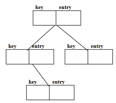
What is Hashing?

We use hashing as a method to implement an existing data structure. The methods- find, insert and remove of table will get of constant time.

In Hashing, we will internally use array. It may be static or dynamic. But we will not store data in consecutive locations. We calculate their storage place using the key and a hash function.

Hash function is a mathematical function that processes on the key to find a certain index in the array of data.

Keys and entries are scattered throughout the array. We will pass this key to the hash function which will return an integer. This number will be used as array index. We will insert the data of the employee at that index.

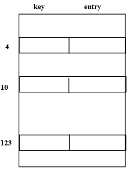
• Insert method will calculate place of storage and insert in TableNode.
• Find method will calculate the place of storage and retrieve the entry.
• Remove method will calculate the place of storage and set it to null.

Examples of Hashing

With the help of examples, you’ll easily understand the working of find, insert, and remove methods.

Suppose we want to store some data and we’ve a list of fruits. The string provides the names of the fruits. The key is the name of the fruit. We’ll pass it to the hash function to get the hash key.

Consider, we got following result from hash function:

hashCode ("apple") = 5
hashCode ("watermelon") = 3
hashCode ("grapes") = 8
hashCode ("cantaloupe") = 7
hashCode ("kiwi") = 0
hashCode ("strawberry") = 9
hashCode ("mango") = 6
hashCode ("banana") = 2

So, we can see that hash function is giving random numbers. We will use these numbers as indices in the array.

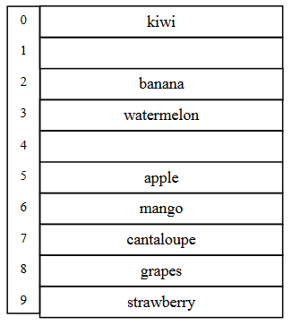
We store the data depending on the indices got from the hashCode. The size of array is 10. This array will be the private part of the data and user will not know about this. So, we’ll inert, find, and remove data using these fruit names.

table[5] = "apple"
table[3] = "watermelon"
table[8] = "grapes"
table[7] = "cantaloupe"
table[0] = "kiwi"
table[9] = "strawberry"
table[6] = "mango"
table[2] = "banana"

We store the data using the hash function which provides us the array index. As we’re retrieving data using names, so we can write them as follows: –

table["apple"]
table["watermelon"]
table["grapes"]
table["cantaloupe"]
table["kiwi"]
table["strawberry"]
table["mango"]
table["banana"]

We are using the integer indices using the hashCode. Here we have used the fruit names as indices of the array. We call it associative array.

If the keys are strings, the hash function is some function of the characters in the strings. One possibility is to simply add the ASCII values of the characters. Suppose the mathematical notation of hash function is h. It adds all the ASCII values of the string characters. The characters in a string are from 0 to length – 1. Then it will take mod of this result with the size of the table. The size of the table is actually the size of our internal array. Mathematically:

   

Example: h(ABC) = (65 + 66 + 67) % TableSize

For each character we have a different bit pattern.

C++ code of hashCode

int hashCode( char* s ) {
    int i, sum;
    sum = 0;
    for(i=0; i < strlen(s); i++ )
        sum = sum + s[i]; // ascii value
    return sum % TABLESIZE;
}

The return type of hashCode function is an integer and takes a pointer to character. Strlen() calculates the length of the string. We run a loop from 0 to length – 1. In the loop, we start adding the ASCII values of the character.

NOTE: That’s not the only way of implementing the hash function. There may be other implementations of hash functions.

Another possibility is to convert the string into some number in some arbitrary base b (b also might be a prime number). The formula is as:

   

Example:

   

• T = Size of the table
• b = Any prime number

Consider, b = 7 and we want the hash value of ABC: –

   

PROBLEM: If the keys are integers, key%T is generally a good hash function, unless the data has some undesirable features. For example, if T = 10 and all keys end in zeros, then key%T = 0 for all keys.

Problems in Hashing

Collision

When two values hash to the same array location, this is called a collision.

Collision takes place when two or more keys (data items) produce the same index. Consider the following scenario: –

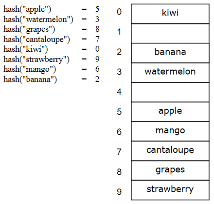
Suppose we want to add another fruit “honeydew” in Figure-5. When we passed “honeydew” to the hash function, it returned “6”.

hash(“honeydew”) = 6

But we already have “mango” at position 6.

We normally treat collisions as a “first come, first served” phenomenon, where the first value that hashes to the location gets it. You have to find something to do with the second and subsequent values that hash to the same location.

We can adopt various solution to encounter this problem.

Solution No. 1

Search for an empty location.

• Can stop searching when we find the value or an empty location.
• Search must be wrap-around at the end.

Keep in mind that in hashing, we do not store data at consecutive positions. Rather, data is scattered. We’ll store the item at the empty location.

Solution No. 2

Use a second hash function.

• …and a third, and a fourth, and a fifth, …

You’re right. Here’s the corrected version in active voice:

If one function returns the same value as the previous one, choose another hash function that implements a different method and returns a different value.

Solution No. 3

Use the array location as the header of a linked list of values that hash to this location.

Our array will be an array of pointers to TableNode. We will create a list node and store the data in it.

Now we will see how we can implement the methods of Table and Dictionary ADT using the hashing function.

Linear Probing

We scan the array sequentially (with wrap-around) in search of an empty cell; we call this collision resolution strategy linear probing.

When there is a collision, we try to find some other place in our array. This approach of handling collisions is called open addressing; it is also known as closed hashing.

More formally, cells at h0(x), h1(x), h2(x), … are tried in succession where hi(x) = (hash(x) + f(i)) mod TableSize,            with f(0) = 0

We’ll understand this through an example. Consider the table of birds given in Figure-6.

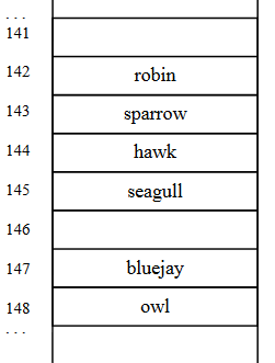
We found these birds at location 142, 143, 144, 145, 147, and 148. When we tried hashCode(“seagull”) = 143, it resulted the location where “sparrow” is present. To place this seagull, we’ll look for the empty place in the table. For this, we’ll perform increment the location of seagull and will continue to increment until we don’t get the empty location to place this seagull. Finally, we found location 145 for this.

When we don’t find an empty place after a linear search, we search the array again from the start, calling this wrap-around. In this case, we treat the array as a circle where the tail connects to the head.

From Figure-6, we see that the last location of array is 148. And hashCode(“cardinal”) resulted “147”. We know that after incrementing 147, we see 148 which is also not empty. For this, searching will start from the top and will continue to come down of the table until no empty place is found.

Problem in Linear Probing

If an item is placed in array[hash(key)+4], the item just before it is deleted. How will probe determine that the “hole” does not indicate the item is not in the array? We may have three states for each location as:

• Occupied: It is filled with some legal data and is occupied.
• Empty (never used): It is empty (never used) and has no data in it.
• Deleted (previously used): It had some data which is now deleted and currently it is empty.

If we delete an element from the chain, how can we know that it was previously filled? When we tried to add “seagull”, it resulted 143. Then we incremented to 144 (already filled) and then finally reached 145 where we placed it. Now, suppose we delete a bird “hawk”, present at position “143” in Figure-6. After deletion, the spot becomes empty. If we try searching for “seagull”, we find this spot empty. So, the problem comes how we would know that something was there at 143.

One problem with linear probing technique is the tendency to form “clusters”.

Clusters

Suppose we want to add another bird in Figure-6. Its hash function returned 143. And we already have three items collided at 143, and we placed two of them at 144 and 145 (for hawk and seagull respectively). So, we’ll insert this new data item at 146. You can imagine if we continue having items that collide at specific location. Then, incrementing each of them is time consuming and cause inefficiency. This is called clustering.

To avoid the problem of clusters, we can use quadratic probing. We won’t go into much detail of it.

Quadratic Probing

• Use F(i)=I^2 (square of i) to resolve collisions.
• If hash function resolves to H and search in cell H is inconclusive, try H+1^2, H+2^2, H+3^2, …

Link List for Collision Resolution

In this, each table position is a linked list. When we are going to insert new data, we will insert the keys and entries anywhere in the list (front easiest). See Figure-7.

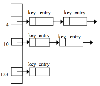
The left vertical array in Figure-7 contains the pointers in it. When we insert the first item, we attach a list node. In the event of a collision, we insert the new item at the start of the linked list.

Link List and Open Addressing Comparison

• Advantages over open addressing:
  • Simpler insertion and removal
  • Array size is not a limitation
• Disadvantage
  • Memory overhead is large if entries are small.

The problem in linear probing is that when our array is full what we should do. This problem can be solved using the link list.

Applications of Hashing

• Compilers use hash tables to keep track of declared variables (symbol table).
• A hash table can be used for on-line spelling checkers — if misspelling detection (rather than correction) is important, an entire dictionary can be hashed and words checked in constant time.
• Game playing programs use hash tables to store seen positions, thereby saving computation time if the position is encountered again.
• Hash functions can be used to quickly check for inequality — if two elements hash to different values they must be different.

When hashing is suitable?

• Hash tables are very good if there is a need for many searches in a reasonably stable table.
• Hash tables are not so good if there are many insertions and deletions, or if table traversals are needed — in this case, AVL trees are better.
• Hashing slows down operations that require sorting the entries.
  • e.g. Find the minimum key

REFERENCE: CS301 Handouts (page 452 to 471)