Binary Search and Linked List for Table ADT

Introduction

In this article, we’ll learn about binary search on the array. And also get the idea about the linked list. We’ve already discussed the effect of sorted and unsorted arrays on the operations of Table ADT (abstract data type). Here, we’re concerned about more implementations of Table ADT i.e. through binary search and linked list. The main reason of studying these things is to gain maximum efficiency in terms of speed and space.

Binary Search

• Binary search is like looking up a phone number or a word in the dictionary.
• Start in middle of book.
• If the name you’re looking for, comes before names on the page, search in the first half.
• Otherwise, look into the second half.

Algorithm for Binary Search

if(value == middle_element)
    value is found
else if(value < middle_element)
    search left half of list with the same method
else
    search right half of list with the same method

Let’s look at the examples of binary search. Consider “a” is an sorted array in ascending order. We’ll discuss three cases in these examples:

• Case 1: value == a[mid]
• Case 2: value > a[mid]
• Case 3: value < a[mid]

Examples of Binary Search

Example No. 1 (Case 1)

Case 1: val == a[mid]

val = 10

low = 0, high = 8

mid = (0 + 8) / 2 = 4

In Figure-2, we’re searching for value (val) “10”. Through median formula [(low+high)/2], we jump to the middle position of the array. Fortunately, we found, what we were looking for, there. The program will stop here and return the value that we found at a specific position.

Example No. 2 (Case 2)

Case 2: val > a[mid]

val = 19

low = 0, high = 8

mid = (0 + 8) / 2 = 4

new low = mid + 1 = 5

If the value is greater than the value at the mid. Then, we’ll look into the upper half of the array. This makes searching very fast, as we don’t have to look whole array rather a small section of the array. We do this by bringing “low” next to the mid. We continue doing this, until “val” is greater than the element in the middle of array.

Example No. 3 (Case 3)

Case 3: val < a[mid]

val = 7

low = 0, high = 8

mid = (0 + 8) / 2 = 4

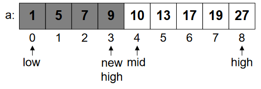
new high = mid – 1 =5

In this, we’ve to look the lower half of the array, If  val < a[mid]. We change the position of “high” and bring it to the one step back from the mid. It can be well understood through figures.

Let, we’re looking for val=7, which is less than mid(10). We’ll continue parsing the array until we don’t reach “7”.

In Figure-7, we finally found 7 at the position 2.

Binary Search _C++ Code

Now, you can understand the binary search code easily.

int isPresent(int *arr, int val, int N){
    int low = 0;
    int high = N - 1;
    int mid;
    while ( low <= high ){
        mid = ( low + high )/2;
        if (arr[mid] == val)
            return 1; // found!
        else if (arr[mid] < val)
            low = mid + 1;
        else
            high = mid - 1;
    }
return 0; // not found

Efficiency of Binary Search

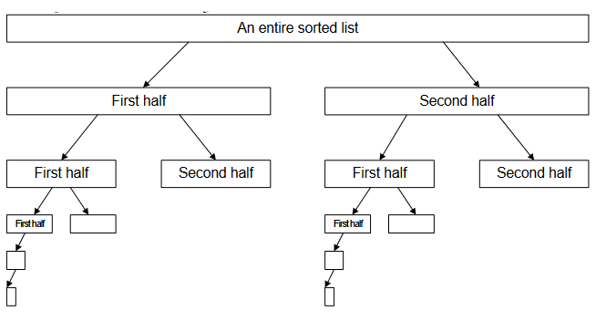
See Figure-8, the search divides a list into two small sub-lists till a sub-list is no more divisible.

When we divide the array of N items into two halves continuously, then:

After 1 bisection, No. of items:

After 2 bisections:

For i bisections, we are left with following no. of items:

Which is at one point of time is only one element of the array.

Computing the value of i from this, gives us:

Linked List

We study the next implementation when we find the problem in previous one. 😊

Binary search made the find operation very fast in array. But in case of insertion or removal, we need to perform shifting of elements. If it’s in middle, then all the elements next to it will be shifted. Worse is at the beginning where shifting will be performed on all the elements of array. So, it’s not good in case of speed for insertion and removal.

The data structure which takes contiguous space in the memory, can cope the above problem. This data structure is the linked list.

Binary search only works for the array.

Nodes of the linked list are scattered over the memory. So, binary search won’t work with them.

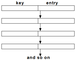
TableNodes are stored consecutively (unsorted or sorted).

• Insert: In case of unsorted linked list, adding the node to front will take constant time. But in case of sorted, you’ve to traverse the linked list for right position of new node.
• Find: All the keys are scanned through whether they are sorted and unsorted. So, time of find is proportional to N.
• Remove: We’ve to perform find first. Later, remove and the links are readjusted accordingly.

Fixed size of the array becomes a constraint and it can’t let more elements in it. While linked list has no such constraint. But the find operation in linked list becomes very slow.

We can optimize the linked list to the skip list to get rid of the problem of slow searching.

Conclusion

We can operate table ADT through binary search for fast find operation. And linked list to avoid the constraint of limited elements. Binary search gets the advantage of fast searching over linked list. But fails in terms of insertion and removal. While linked list take over binary search in terms of insertion and removal. Moreover, linked list can be optimized for fast find operation through skip list.

REFERENCE: CS301 Handouts (page 430 to 438)