Introduction
We ran out a problem related to time while using selection, insertion, and bubble sort. Where, we were heading to the time consumption of n^2, n = no. of elements in array. But we can upgrade it to the following time: –
[latex]\[N{\log _2}(N)\][/latex]You can see Figure-1 that proves the inefficiency of n^2 method.
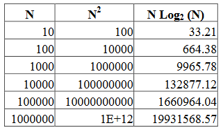
Divide and conquer strategy will help us to attain this proficiency.
Three types of sort that use divide and conquer strategy: –
- Merge sort
- Quick sort
- Heap sort
In this article, we’ll expand the details of merge and quick sort.
Divide and Conquer
Divide and Conquer: Break things into the small sections (divide), and solve each section separately (conquer).
To better understand this, see the example given below: –
Here is the full array: –

Divide it into small sections: –

Sort each section separately: –

Final conquest: array is sorted.

Analysis of Divide and Conquer Method
- To sort the halves approximate time is (n/2)^2+(n/2)^2.
- To merge the two halves approximate time is n.
- So, for n=100, divide and conquer takes approximately:
- = (100/2)^2 + (100/2)^2 + 100
- = 2500 + 2500 + 100
- = 5100
And we know 5100 < (n^2 = 10,000).
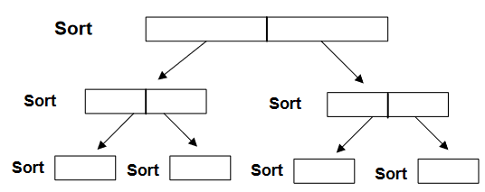
We’ll divide the list into 2 parts and each part in subdivided into further sub-parts. At the end, we’re left with single element or maximum two elements. If we’ve 2 elements at the end, we can sort them using a single if statement. See Figure-6: –
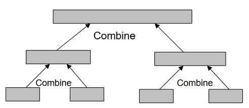
After sorting each section, we’ll merge them, shown in Figure-7: –
Merge Sort
Merge sort is a divide and conquer algorithm that does exactly what we’ve discussed above.
- It splits the list in half.
- Merge sorts the two halves.
- Then merges the two sorted halves together.
- Merge sort can be implemented recursively.
Steps in Merge Sort
- If the number of items to sort is 0 or 1, return.
- Recursively sort the first and second halves separately.
- Merge the two sorted halves into a sorted group.
Merge Sort through Figures
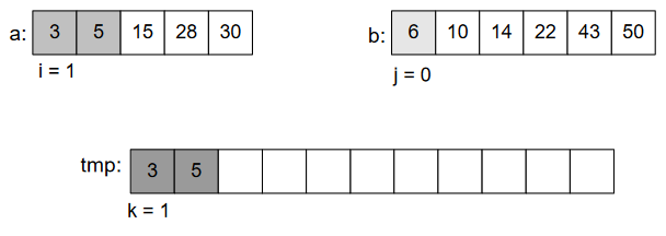
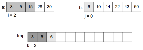
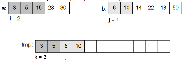
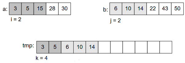
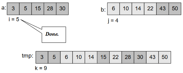
In the below figures, we’ve 2 sections of an array, each is sorted. We’ll fill the 3rd array with sorted elements of those 2 sections.
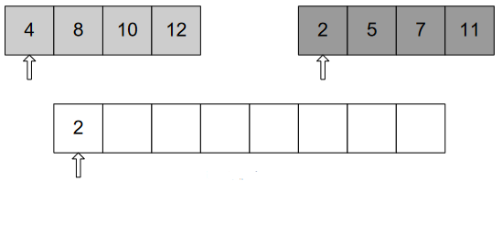
In Figure-8, three pointers pointing to the beginning of three arrays, each pointer for a specific array. After comparing elements of those two sections, we put into 3rd array according to the order of element. As 2<4, put 2. And forward the pointer to next element shown in Figure-9.
As 4<5, put 4 and move the pointer ahead.
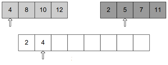
We’ll continue doing this, until we get the whole array sorted.
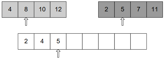
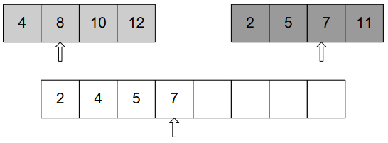
Obviously, this splitting of array will be possible through recursion. Where, at the end, we’re left with 2 elements and we perform comparison to sort them. And finally merge those parts to get final sorted array.
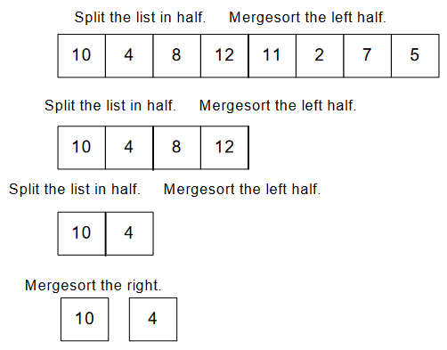
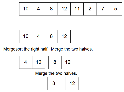
Now, merging 3rd layer: –
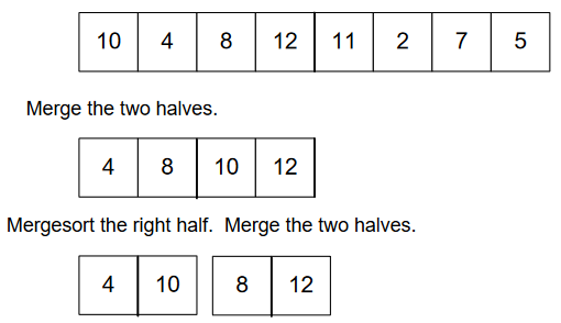
It’s not over, we still have half of the array 😊. Go with the same procedure.
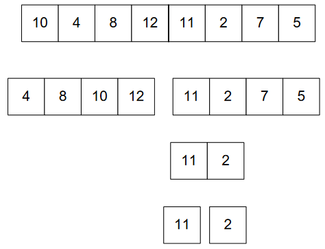
Sort them.
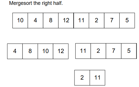
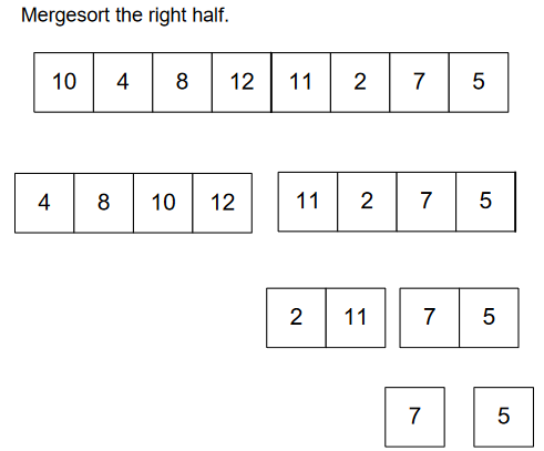
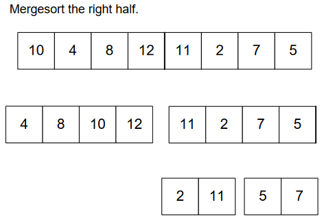
We’re almost done. 😊
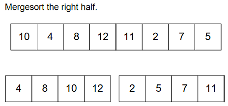
Finally, we got our sorted array. 🎉

C++ code for Merge Sort
void mergeSort(float array[], int size){
    int * tmpArrayPtr = new int[size];
    if (tmpArrayPtr != NULL)
        mergeSortRec(array, size, tmpArrayPtr);
    else{
        cout << “Not enough memory to sort list.\n”);
        return;
    }
    delete [] tmpArrayPtr;
}
void mergeSortRec(int array[], int size, int tmp[]){
    int i;
    int mid = size/2;
    if (size > 1){
        mergeSortRec(array, mid, tmp);
        mergeSortRec(array+mid, size-mid, tmp);
        mergeArrays(array, mid, array+mid, size-mid, tmp);
        for (i = 0; i < size; i++)
            array[i] = tmp[i];
    }
}
To understand this code, sync it with the following figures. Means, below images clear what’s happening in the above code.

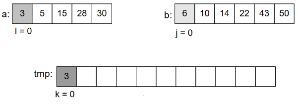
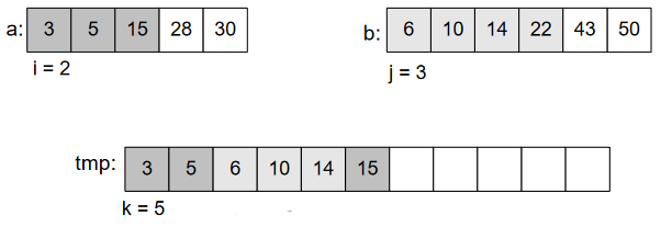
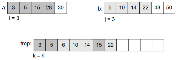
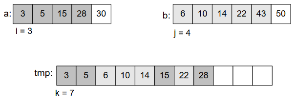
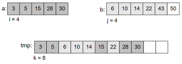
Finally, we did it. 😊
Merge Sort and Linked List
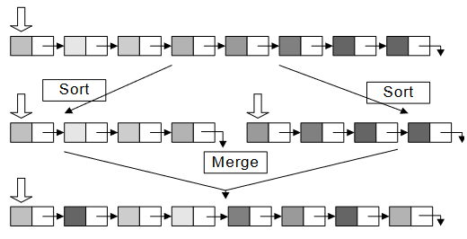
Merge sort works with arrays as well as linked lists.
Merge Sort Analysis
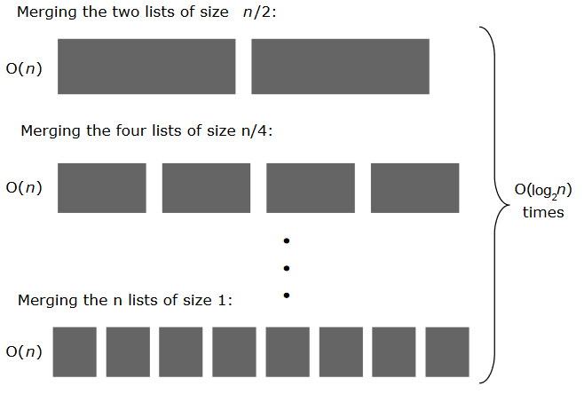
- Time gets shorter as compared to the selection, insertion, and bubble sort.
- Merge sort requires O(n) extra space for merging.
Quick Sort
Quick sort is another divide and conquer algorithm.
Quick sort is based on the idea of partitioning (splitting) the list around a pivot or split value.
You can better understand quick sort through examples: –
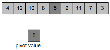
Swap pivot value with last element of the array, Figure-35: –
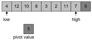
In Figure-36, we’ve two indexes: low, high. “low” starts from 0th position and goes towards right until (n-1)th position. On the other hand, “high” starts from (n-1)th position and move towards left until 0th position. Our main focus is “low should be greater than pivot element and high should be less than pivot”.
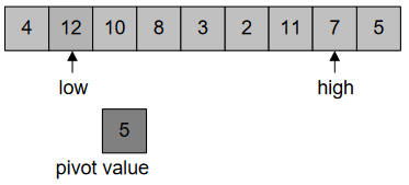
“low” stops at 12, as it’s greater than pivot 5, Figure-36: –
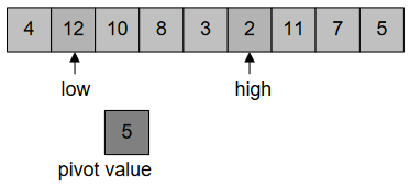
“high” stops at 2, as it’s less than pivot 5, Figure-37: –
After this, we’ll swap these values at “low” and “high”, Figure-38: –
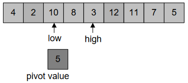
We’ll continue pointing “low” to greater value and “high” to the less value than pivot value. And swapping them, until they (low and high) don’t cross each other.
After swapping low=10 and high=3, we get this, Figure-39: –
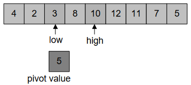
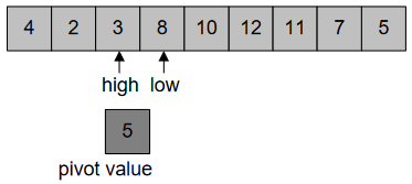
In Figure-40, when “high” and “low” cross each other, swap the index with pivot. Swapping of index is shown in Figure-41: –

Figure-42, this array isn’t sorted yet, but element 5 has found its destination. The numbers on the left of 5 are smaller while on the right, they’re greater than it.

We can perform recursion in quick sort to make the whole array sorted.
C++ Code for Quick Sort
void quickSort(int array[], int size){
    int index;
    if (size > 1){
        index = partition(array, size);
        quickSort(array, index);
        quickSort(array+index+1, size - index-1);
    }
}
int partition(int array[], int size){
    int k;
    int mid = size/2;
    int index = 0;
    swap(array, array+mid);
    for (k = 1; k < size; k++){
        if (array[k] < array[0]){
            index++;
            swap(array+k, array+index);
        }
    }
    swap(array, array+index);
    return index;
}
Conclusion
Divide and Conquer strategy helped to attain the proficiency in terms of speed and space. In selection, insertion, and bubble sort; sorting time was n^2. But the advantage was there in terms of space. Means, no extra space was required for the sort operation. While in case of divide and conquer sorting techniques, we upgraded the time to: –
[latex]\[N{\log _2}(N)\][/latex]In case of space for divide and conquer; merge sort was taking extra space while quick sort doesn’t take the extra space. So, quick sort wins both in case of time and space. 🥳
REFERENCE: CS301 Handouts (page 485 to 504)


